Introducing Cohorts

Cohorts is a Python library for managing, analyzing and plotting clinical and genetic data from patient cohorts. It was spun out of our work analyzing data from clinical trials of checkpoint blockade in melanoma, lung, and bladder cancer. The sponsors of these trials typically collect a wide range of data for each patient in order to discover and evaluate potential biomarkers for association with benefit from therapy. While some aspects of Cohorts are specific to that context (e.g. the integration with neoantigen prediction), other components are more generally usable.

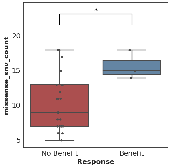
A prototypical use case for Cohorts is a Mann-Whitney comparison and associated box plot of the number of missense SNV mutations found in patients who did benefit from therapy (where benefit is defined by the user, e.g. progression-free survival greater than 6 months) versus those who did not benefit.

In its simplest form, this looks like:

cohort.plot_benefit(on=missense_snv_count)

But where does this cohort come from, what is this missense_snv_count, and what else can we plot? Let’s explore how Cohorts works!

Note: all code in this post is available in a Jupyter notebook.

Creating a Cohort

A cohort must be populated before analysis and plotting can proceed. Within Cohorts, each Cohort consists of a set of Patients, each of whom may have tumor and normal Samples.

Samples hold paths to associated BAM files as well as Cufflinks or kallisto output. Patients contain key clinical variables (clinical benefit status, overall survival, progression-free survival, deceased status, progression status), tumor and normal Samples, paths to tumor-normal VCFs, HLA alleles, as well as any additional relevant data. Cohorts contain all Patients as well as a variety of cohort-level settings.

Patients do not need to contain Samples, and they won’t when used for purely clinical data analyses. If you have data that isn’t easily modeled as described, but would like to make use of Cohorts, please file an issue on GitHub!

Analyzing a Cohort

The analysis and plotting functions of Cohorts generally rely on Pandas DataFrames. The simplest way to begin analysis is via direct access to the DataFrames that Cohorts produces. For example:

df = cohort.as_dataframe()

To go further, Cohorts will enhance user-provided data by calling out to external libraries like Topiary, Varcode and Isovar. These results are then exposed as potential biomarker datapoints for analysis.

For example, the function missense_snv_count, which requires paths to SNV VCF(s) to be specified in the Patients, utilizes Varcode to filter those mutations to those that are missense. neoantigen_count uses Topiary to compute predicted neoantigens from those SNVs.

These functions can be plugged into Cohorts:

# Return a DataFrame with "neoantigen_count" as a column,
# in addition to user-specified patient data.
df = cohort.as_dataframe(on=neoantigen_count)

# Return a DataFrame with "Neoantigen Count" and
# "Missense SNV Count" as additional columns.
df = cohort.as_dataframe(on={"Neoantigen Count": neoantigen_count, "Missense SNV Count": missense_snv_count})

While a number of these data-enhancing functions are available out of the box, users can always write their own custom functions to support their analyses of interest.

Below is a simple custom function example:

def smoker_or_senior(row):
    return row["smoker"] == True or row["age"] >= 65

This can be used just like the functions above:

df = cohort.as_dataframe(on=smoker_or_senior)

Plotting

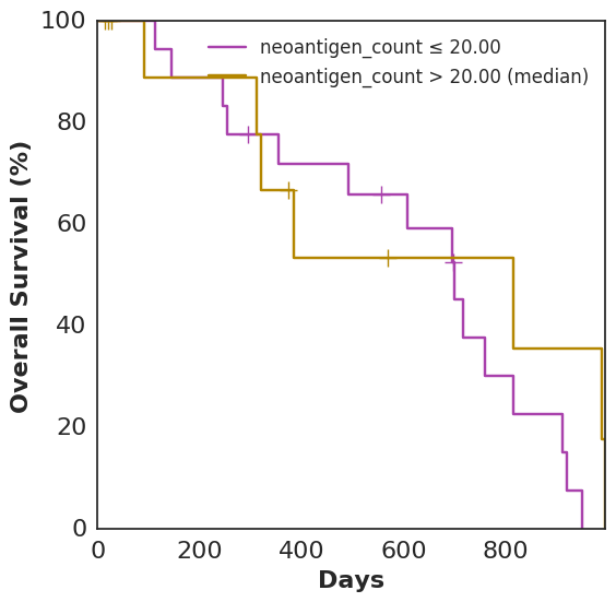
In addition to plot_benefit, Cohorts comes with various analysis and plotting functions. To name a few: plot_survival, plot_correlation, coxph, and bootstrap_auc. plot_survival uses Lifelines to plot two survival curves split by a specified variable. The following code generates a survival curve for patients with more neoantigens than the median and a survival curve for patients with fewer, based on Topiary’s neoantigen prediction:

cohort.plot_survival(on=neoantigen_count)

Analyses and plots based only on data supplied directly to the Patient, as opposed to computed features using data-enhancing functions, are also fair game:

# note: resultant image not shown here
cohort.plot_survival(on="smoker")

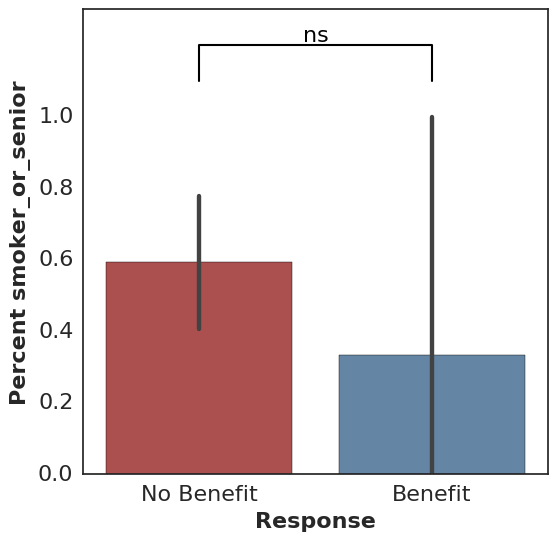
For binary features, Fisher’s exact test is used along with an associated bar plot:

cohort.plot_benefit(on="smoker")

All calls to plot_benefit result in a p-value significance indicator at the top of the plot, thresholded by 0.05 by default (* for significant and ns for not significant).

Results from other data locations can be loaded into an analysis using join_with:

# note: resultant images not shown here
cohort.plot_benefit(on="PD-L1 Expression", join_with="pdl1")
cohort.plot_correlation(on={"Missense SNV Count": missense_snv_count,
                            "PD-L1 Expression": "PD-L1 Expression"},
                        join_with="pdl1")

The above uses a DataFrameLoader, which is defined when a Cohort is created. It associates "pdl1" with a given DataFrame and specifies how to join that DataFrame with the Cohort. We typically load results from IHC analysis, tumor clonality estimates, mutational signature deconvolution, and TCR-Seq in this way. While extra data sources can also be added to the Cohort data itself to avoid joining (see Patient.additional_data), keeping certain data sources separate is helpful when a data source has a one-to-many relationship with the Cohort or is slow to load.

Consistency and Reproducibility

Many of the features in Cohorts have a goal of promoting consistency and reproducibility across various analyses. Examples include:

Variant Filtering

A user can define custom variant filtering functions, and filter variants accordingly. For example:

# Filter variants to those with at least 3 reads in the tumor sample.
def tumor_read_filter(filterable_variant):
    somatic_stats = variant_stats_from_variant(
        filterable_variant.variant,
        filterable_variant.variant_metadata)
    return somatic_stats.tumor_stats.depth >= 3

# Use a default filter function for the Cohort.
# note: resultant images not shown here
cohort.filter_fn = tumor_read_filter
cohort.plot_survival(on=missense_snv_count)

# ...or specify a filter function ad-hoc.
cohort.plot_survival(on=missense_snv_count,
                     filter_fn=alternative_filter)

Data Caching and Provenance

Cohorts caches many results, such as variant effects and predicted neoantigens, to mitigate the computational overhead frequently involved. A file-based approach enables easy sharing and manipulation of cached objects.

Cohorts also keeps track of the context in which the cache was generated by tracking the versions of software used to generate the cache. This context, as well as a hash of the base (unenhanced) data, is available for printing and optional version checking.

Other Resources

Ready to take Cohorts for a spin? The following notebooks should help you get started:

• Example code from this post
• Quick-start - using Cohorts with TCGA data
• Part I - Creating a cohort from clinical data
• Part II - Creating a cohort from clinical & SNV data

We’d love to hear from you if you have any feedback, suggestions, or bug reports!